We Gaussianized the Reference: Repairing Evaluation for Multimodal Filters
A full-density audit repaired grid semantics, boundary checks, and scalable reference inference—then showed which nonlinear-filter rankings survived.
Series: VBF Experiments, August 2026
Contents
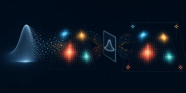
The previous nonlinear-filtering experiments had an awkward asymmetry. The reference filter was a complete probability distribution on a scalar grid, but several headline diagnostics reduced that distribution to a mean and variance before scoring it. We had built a multimodal reference and then asked it to behave like a Gaussian.
That does not mean every old number was wrong. The learned Gaussian-mixture state NLL was already evaluated under the complete learned mixture, and its ranking survives this audit. But reference state scores, interval calibration, and shape comparisons did not consistently use the complete grid density. We also lacked forward KL, CDF distances, basin-mass diagnostics, and hard checks for probability leaking into the edge of the finite grid.
This note is about repairing that evaluation before starting a more ambitious project on controlled posterior projection. The result is reassuring and inconvenient at the same time:
The strongest state-density anchor remains the strongest, but none of the current filters is close to nominal 90% highest-density-set coverage.
The implementation lives in
dwrtz/ml-examples, alongside a
full evaluation report
with the metric definitions, commands, and numerical checks behind this note.
What “Gaussianized the reference” means#
The scalar reference filter represents a filtering belief with grid-point probability masses \(p_g\). Those masses sum to one. They are not density values. On a uniform grid with spacing \(\Delta z\), the corresponding density at a grid point is approximately
\[ p(z_g) \approx \frac{p_g}{\Delta z}. \]This distinction matters immediately for state log score. If the realized state is \(z_t^{\mathrm{true}}\), we should interpolate the grid log density and report
\[ -\log p_t(z_t^{\mathrm{true}}), \]not the negative log of a grid-cell mass and not the log density of a Gaussian with the reference mean and variance.
It also matters for KL. Given a continuous approximate density \(q(z)\), we first convert it to conditional grid masses:
\[ \widetilde q_g = \frac{q(z_g)\Delta z}{\sum_j q(z_j)\Delta z}. \]Then the finite-grid forward KL is
\[ D_{\mathrm{KL}}(p\Vert q) \approx \sum_g p_g\left(\log p_g-\log\widetilde q_g\right). \]There is no second factor of \(\Delta z\) after both distributions have been converted to normalized masses. Mixing these two conventions is an easy way to produce a plausible-looking but grid-resolution-dependent metric.
The repaired evaluator now reports:
- interpolated reference state log density;
- forward and reverse KL on the common grid;
- Cramér and Wasserstein-1 distances from complete CDFs;
- exact grid predictive-observation evidence;
- 50%, 80%, 90%, and 95% highest-density-set coverage, length, and number of disconnected intervals;
- PIT calibration and KS distance, including observation-strength regimes;
- mass error across the periodic \(2\pi\) basins;
- episode-level tail risk for state NLL and forward KL.
The highest-density-set point is especially important. A multimodal 90% set can be several disconnected intervals. A mean-plus-or-minus-width interval is a different object, even when both happen to contain 90% probability under a Gaussian.
The reference also had to become scalable#
The old random-walk predictor materialized a dense \(G \times G\) transition matrix. That is a fine oracle for small tests, but its time and storage scale quadratically with grid size. Future controller experiments need to reuse the physical reference across many approximate action rollouts, so quadratic grid prediction would become the bottleneck before the interesting work began.
For random-walk dynamics,
\[ z_t=z_{t-1}+w_t,\qquad w_t\sim\mathcal N(0,Q), \]prediction on a uniform grid is Gaussian convolution. The production code now uses a truncated banded convolution for narrow kernels and a zero-padded FFT convolution for wide kernels. For AR(1) dynamics, it first conservatively pushes mass through \(z \mapsto az\), then applies the same Gaussian convolution. The dense transition remains only as a small-grid correctness oracle.
The cache changed with it. A reference artifact now records predictive and
filtering log mass, exact predictive evidence, moments, channel data,
boundary diagnostics, implementation and semantics versions, and precision.
When an audit uses saved physical episodes, the exact x/y/z batch is
fingerprinted into the cache key. That last detail prevented a subtle mistake:
regenerating the same JAX seed under float64 does not necessarily reproduce the
same trajectory sampled under float32.
The first guardrail failure was useful#
The four legacy anchors used a 1,601-point grid on [-16, 16]. The first audit
run failed before producing a comparison: the maximum right-edge filtering mass
was \(1.615 \times 10^{-4}\), above the float32 limit of \(10^{-4}\).
The fix was not to relax the tolerance or clip the distribution. The audit
expanded to a 2,049-point [-24, 24] screening grid. The maximum
filtering or predictive edge mass then fell below \(5.6 \times 10^{-8}\), with no
realized states outside the grid.
This is exactly why numerical-integrity fields belong beside scientific metrics. A state NLL can look perfectly ordinary while the finite support is quietly deciding the tails.
What the four-anchor audit says#
This first repaired audit uses one saved training seed, one paired evaluation seed, 128 episodes, and 96 steps. It is a reproducible anchor check, not the larger multi-seed confirmation protocol.
| Anchor | State NLL | Forward KL | W1 | HDS 90% | PIT KS | Basin TV | Predictive-y NLL |
|---|---|---|---|---|---|---|---|
| K2 FIVO bridge | 3.3139 | 1.3754 | 1.8029 | 0.6835 | 0.1973 | 0.2014 | 0.7809 |
| K3 joint IWAE | 6.0436 | 4.0847 | 3.8283 | 0.4291 | 0.5040 | 0.4465 | 0.7659 |
| K3 hybrid IWAE/projection | 4.7932 | 2.8253 | 3.3112 | 0.5289 | 0.4170 | 0.3505 | 0.7703 |
| K2 Power-EP | 16.8500 | 13.7381 | 2.4885 | 0.5124 | 0.2835 | 0.3734 | 0.5267 |
Lower is better except HDS coverage, whose target is 0.90.
The ranking story is unusually clean:
- K2 FIVO bridge is best on state NLL, forward KL, Wasserstein-1, HDS calibration, PIT, and periodic-basin mass.
- Power-EP is best on predictive-y NLL, but worst on state NLL and forward KL.
- The K3 hybrid sits between FIVO bridge and K3 IWAE on the state-density measures.
The repaired metrics therefore preserve the existing role assignment. They also sharpen the warning attached to it. FIVO bridge is “best” at 68.4% empirical coverage for a nominal 90% HDS. That is not calibrated; it is merely less miscalibrated than the other current anchors.
Power-EP shows the complementary failure. Its observation prediction is much better, but its forward KL is about ten times the FIVO bridge value. Optimizing for the predictive normalizer can still delete too much state-belief mass.
This extends the conclusion from Strict Nonlinear Filtering With Mixtures, Particles, And Flows and Strict Online Variational Bayesian Filtering: posterior family, proposal, projection, and objective must agree about what the filter is supposed to preserve.
One metric did not behave quietly#
The K2 FIVO bridge was rescored on the same saved physical episodes with a float64 reference and the stricter \(10^{-6}\) edge threshold. State NLL, forward KL, Cramér distance, W1, HDS coverage, PIT, and exact predictive evidence were stable at headline precision.
Reverse KL moved from 4.946 in float32 to 4.733 in float64.
That is not a reason to discard reverse KL. It is a reason to label it secondary. Reverse KL places approximate-belief mass in regions where the reference density may be extremely small, so it is unusually sensitive to finite-grid truncation, density floors, and float32 underflow. Any table that reports it should also report grid range, approximation tail mass, density floor, and precision.
Forward KL is the primary distortion for the next projection-control program because deleting a plausible reference mode is exactly the failure we want to penalize.
The scaling result is about memory, not a universal speed claim#
On a Lambda A10 with batch size 128 and 2,049 grid points, the dense oracle took 0.145 ms per prediction after compilation. FFT took 0.155 ms. Dense matrix multiplication is very good on a GPU, so convolution did not win this isolated latency race.
It did win the scaling argument:
| Method | Compile s | Operator storage | Peak device memory | Max error vs dense |
|---|---|---|---|---|
| Dense | 1.819 | 16.016 MiB | 78.179 MiB | — |
| FFT | 0.337 | 652 bytes | 20.019 MiB | \(6.11 \times 10^{-7}\) |
The FFT representation is about 25,700 times smaller, uses roughly one quarter of the peak device memory, and compiles more than five times faster. More importantly, it does not turn larger grids and nested planner rollouts into a quadratic storage problem.
What this changes next#
The audit did not discover a hidden winner. It established a trustworthy floor for asking the next question:
Can a bounded-memory filter choose when to preserve modes, when to compress, and how much local inference computation to spend based on the future value of the belief it carries?
The first controller experiment should not start with reinforcement learning. The model is known, the action library is finite, and inference actions do not change the passive physical process. A useful next experiment begins with an exact two-hypothesis option-value model and delayed-disambiguation scalar benchmarks, then compares fixed, greedy, full-information rollout, and causal self-rollout policies.
That work would have been difficult to interpret on the old evaluator. Now a controller that preserves an extra mode can be credited through forward KL, HDS structure, basin mass, and tail risk—without asking the reference to pretend it was Gaussian first.
Reproduce the audit#
make check-grid-reference

uv run python scripts/audit_full_density_metrics.py \
  --config experiments/projection_control/full_density_audit/01_current_anchors.yaml \
  --output-dir outputs/projection_control/full_density_audit
The implementation is source commit 3c3dbea,
which contains the evaluation changes described here.
The main source entry points are:
src/vbf/control/grid_beliefs.pysrc/vbf/control/grid_metrics.pyscripts/audit_full_density_metrics.pyscripts/benchmark_grid_prediction.py
For the broader history, start with A Tour of Learned and Reference-Free Bayesian Filters and Amortizing Quadrature Filters Without Losing Calibration.