A Bayesian Filter Repair That Did Not Pass the Full Test
A geometric Gaussian merge removed a large density error within budget. A separate guardrail still failed, while scalar recovery remained unresolved.
Contents
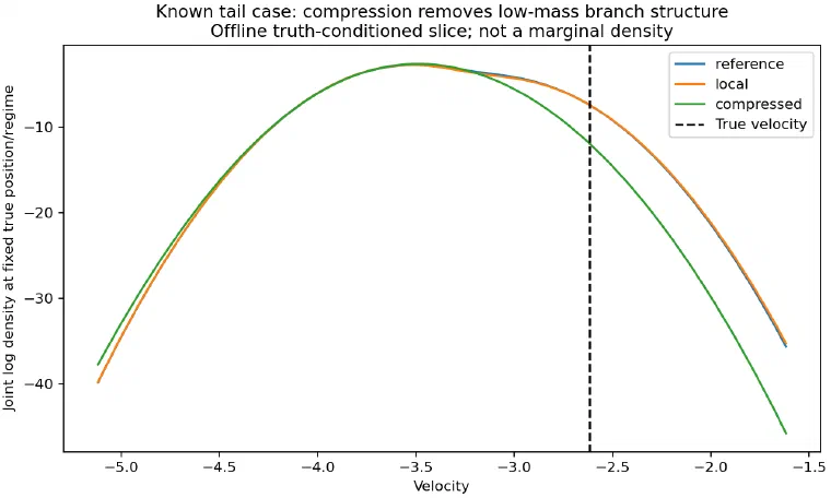
A four-Gaussian Bayesian filter tracked a switching motion model well on average. It also assigned much too little density to the realized state at one observation. We traced that miss to the way it merged Gaussian components, then tested one classical replacement. The large miss disappeared, and the replacement stayed within the time and memory budgets.
We still did not nominate it for confirmation. A separate, previously declared guardrail failed. The increase was small and did not demonstrate material tracking harm, but the rule required every check to pass.
The useful result is the combination: a measured compression mechanism, an intervention that addressed it, and a stopping decision that preserved both the benefit and the remaining failure.
The cover shows the original miss: a slice of joint log density at the realized position and regime. It is an offline diagnostic, not a marginal density or information available to the filter.
First, ask what the observations can reveal#
A Bayesian filter carries a distribution over a hidden state as observations arrive. A bounded filter also has to compress that distribution into a small, fixed amount of memory. Poor results can therefore have different causes: the observations may leave uncertainty unresolved, or the approximation may lose information that a more accurate filter retains.
After our earlier learned-controller experiments, we tested this distinction before investing in another learned method. The study used two matched scalar problems and one independent motion problem. All were simulations with known generative parameters.
In the scalar pair, the hidden state is an unwrapped random walk. The first sensor measures its sine plus Gaussian noise. The second is identical except for one absolute, linear observation at index 12. A sine reading cannot distinguish a state from the same state shifted by a full period; the linear reading breaks that symmetry.
We filtered each stream from three initial priors: \(N(0,8)\), \(N(2\pi,8)\), and \(N(1,8)\). Here the second parameter is variance. There were 16 paired physical episodes, each with 24 observations, process and sensor variances 0.1, and an observation of the initial state at index zero.
The numerical reference recovered from the different priors in 16/16 episodes with the linear probe and 0/16 with only periodic observations. Recovery required normalized Wasserstein distance \(W_1/(2\pi)\) at most 0.05 for three consecutive observations starting at or after the probe, with no later exceedance through the horizon.
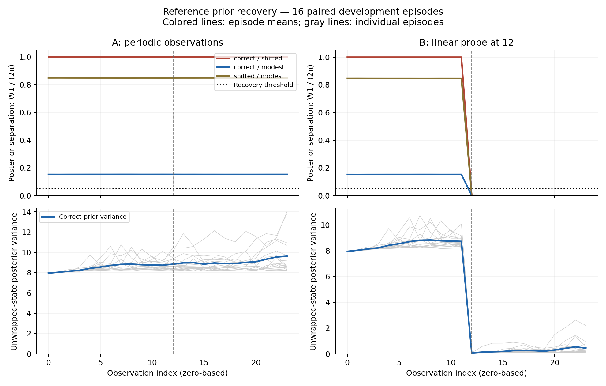
The correctly initialized reference’s postprobe state RMSE was 3.348 for the periodic sensor and 0.394 with the probe. Yet its final uncertainty about the observed sine signal was almost identical. Accurate signal estimation can coexist with substantial uncertainty about absolute location. That uncertainty is part of the task, rather than evidence of a broken filtering implementation.
This conclusion is specific to replacing one sine reading with a linear reading. We did not run an equal-information stronger-sine comparison.
Recovery was possible, but the bounded filters did not always achieve it#
The next comparison used four fixed classical approximations. A single Gaussian used moment matching; mixtures used Gauss–Hermite integration and weighted expectation-maximization updates. K denotes retained component capacity and Q denotes quadrature order. Prediction and the linear observation used analytic Gaussian-mixture operations.
| Method | Recovery to the correct reference after the probe | Correct-prior postprobe RMSE | Correct-prior 90% coverage |
|---|---|---|---|
| Numerical reference | 16/16 | 0.394 | 92.19% |
| Single Gaussian, K1/Q128 | 10/16 | 0.673 | 82.81% |
| Mixture, K4/Q128 | 14/16 | 0.398 | 91.67% |
| Mixture, K4/Q256 | 14/16 | 0.398 | 91.15% |
| Mixture, K8/Q128 | 14/16 | 0.396 | 92.19% |
Recovery requires all three approximate initializations to approach the correctly initialized reference. The accuracy columns use only the correct prior. Their favorable means do not erase failures from other initializations.
Both K4 rows failed on the same two episodes. Doubling quadrature preserved every recovery classification and delay. K8 also recovered in 14/16, with one different failure and a whole-episode median update time of about 1.32 ms on the probe problem, above the provisional 1 ms target.
Agreement among approximations is also insufficient: the single-Gaussian row had eight postprobe observations across three episodes where the different priors agreed but failed the correct-reference proximity test. All censored episodes remain counted. The full scalar recovery table keeps these endpoints separate.
This establishes an approximation limitation under recoverable observations. It does not yet tell us whether the remaining scalar error comes from numerical integration, compression, or information lost earlier in the trajectory.
A motion model made compression easier to isolate#
The independent problem tracks position, velocity, and a hidden acceleration sign from noisy position readings. It uses known linear dynamics, Gaussian noise, a regime-switching probability of 0.03, and acceleration magnitudes 0, 0.125 and 0.25. Each setting has the same 16 paired physical seeds and 256 observations. The first observation follows a state transition.
Conditional on the regime, a Kalman update is analytic. From a four-component carry, branching over the next regime produces at most eight Gaussians. The compression step must reduce them back to at most four. This exposes a clean comparison between an exact local update and the distribution actually carried.
The classical pilot included an interacting multiple-model filter, exact branching followed by moment matching, Gaussian sums, and informed Rao–Blackwellized particle filters. The named long-history reference used 16,384 particles, replicate 0. It passed checks against short exact enumeration, alternative particle budgets and random seeds, and selected deterministic Gaussian-sum references.
The existing K4 Gaussian sum performed well on average. Its mean excess joint log loss was -0.000254 nats per observation at acceleration 0.125 and +0.000518 at acceleration 0.25. It matched the reference’s 101/127 and 108/127 recovered regime changes. These are events within 16 episodes, not 127 independent trials.
But one previously identified observation had 4.511265 nats of excess joint log loss. At that observation, the exact local update had excess -0.007773 nats. Compression itself contributed 4.519038 nats. The four validated reference scores spanned only 0.007944 nats there.
Two rare branches carried about 1.21% of total probability but supplied 99.944% of the exact candidate’s joint density at the realized truth. The existing velocity-bin rule merged them with a much heavier branch. It preserved regime mass, means and covariances while sharply reducing density in that separated region—the effect shown in the cover.
This was a diagnosis of one known episode. Only two observations in that episode exceeded one nat; every other episode maximum at acceleration 0.25 was below 0.5 nats. It was not a discovery of frequent independent tail failures.
One geometric merge rule, tested locally and recursively#
We declared one replacement based on Runnalls’ Gaussian-mixture reduction criterion. It uses an efficiently computed KL bound to select pairs for moment-preserving merges. Our implementation uses full two-dimensional covariances, recomputes eligible pair costs after every merge, and retains at most two Gaussians per regime. It has no truth-dependent merge choice, cross-regime merge, pruning, or probability floor.
Both comparisons matter:
- Common inputs: apply every compressor to the same exact candidate from the unchanged existing K4 filter. Only that original filter advances.
- Self-fed filtering: each method constructs the next candidate from its own preceding compressed belief, so its errors can propagate.
For self-fed runs, define realized excess as \(E_t=\log p_t-\log q_t\), where p is the reference density and q is the carried joint density, evaluated at the realized state and regime. The episode tail sum is
\[ S=\sum_t\max(E_t-1,0). \]On common inputs, replace the reference with the exact local candidate. These are realized log-density contrasts; they are not estimates of KL divergence.
| Acceleration 0.25 | Existing K4 | Runnalls K4 |
|---|---|---|
| Mean episode tail sum, common inputs | 0.224760 | 0 |
| Mean episode tail sum, self-fed | 0.229923 | 0 |
| Maximum episode tail sum, self-fed | 3.678761 | 0 |
| Maximum step excess, self-fed | 4.511265 | 0.412746 |
| Episodes with excess above one nat | 1/16 | 0/16 |
| Median complete update | 0.409 ms | 0.630 ms |
| Maximum retained algorithm state | 2,235 bytes | 2,235 bytes |
Tail sums and excess are in nats. Runnalls grouped the nearby heavy branches together and retained the rare pair as a separate Gaussian on the common candidate. Its own recursive trajectory also removed the large miss.
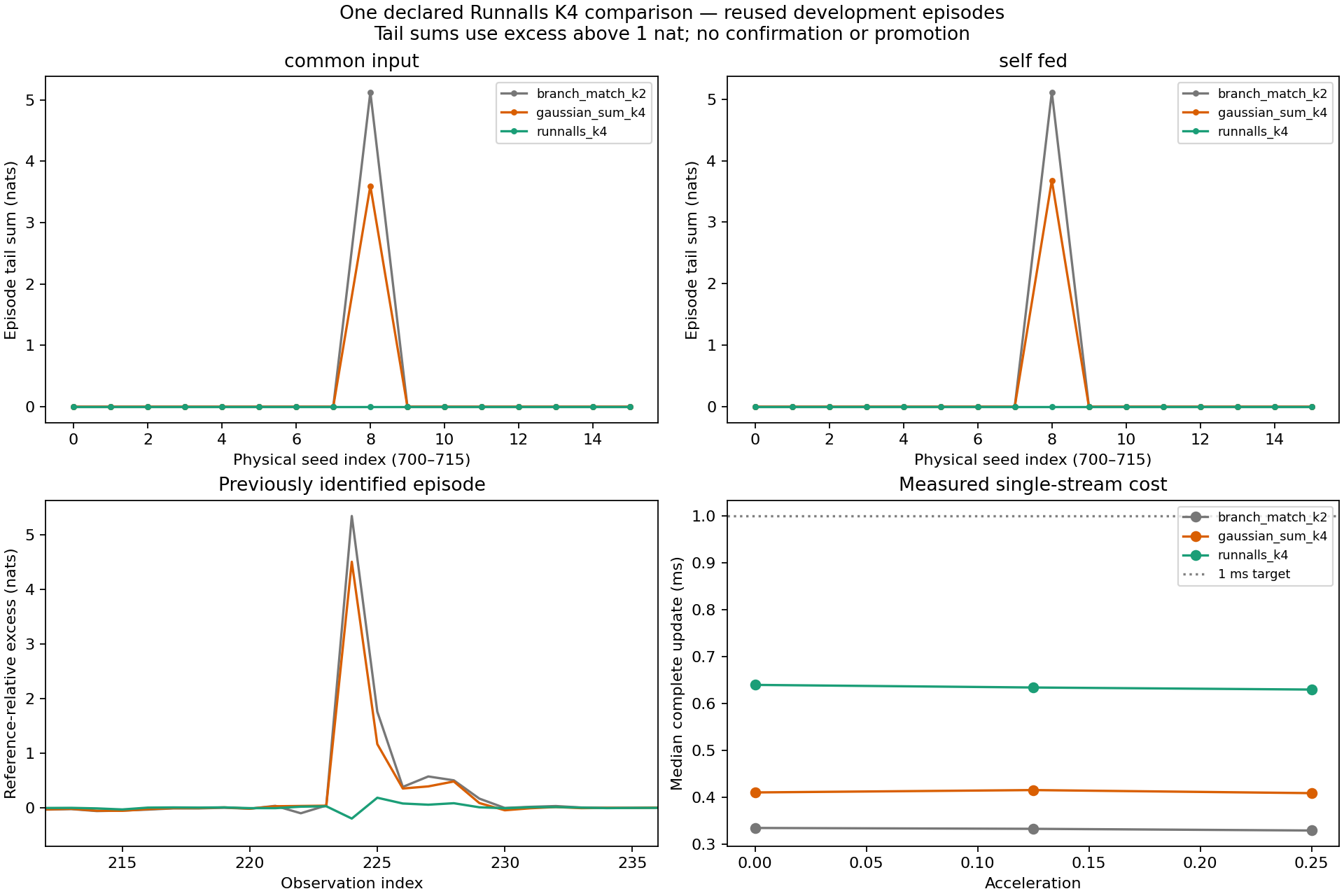
The gray K2 row is native moment matching with one Gaussian per regime. All tail-sum benefit in this comparison comes from the already inspected episode. Tracking and regime recovery remain close to existing K4. Zero observed tail episodes does not establish zero future risk.
Across all settings, Runnalls’ median update was 0.630–0.640 ms, with at most eight branch evaluations and 18 pair evaluations per update. The largest algorithm-state estimate was 2,251 bytes, including the carried belief, model and shared arrays. Temporary payloads and process-wide memory were reported separately; the workspace estimate is not a peak-memory bound. An observed 13.411 ms update remains reported; the median target is not a worst-case latency guarantee.
The check that stopped the experiment#
The frozen decision rule required every screen to pass, including repetition of the positive-acceleration guardrails after excluding the known episode. That exclusion exposed the failure.
At acceleration 0.125, maximum step excess across the remaining 15 episodes rose from 0.195930 to 0.209711 nats. The increase, 0.013782 nats, failed the declared zero-increase margin. All four reference variants gave the same decision. The result was 238 passing gate entries out of 242; the four failures are one guardrail evaluated under four references.
Both maxima are far below the one-nat tail threshold. This was a strict development convention, not an externally validated application tolerance. Its failure does not demonstrate material tracking harm. It does mean the candidate did not satisfy the test we chose before running it.
Average improvements were uncertain too. Paired mean joint-loss differences were +0.000237 nats per observation at acceleration 0.125 and -0.001353 at 0.25; both exploratory simultaneous 95% intervals included zero. Removing the known seed changed the latter mean to +0.000361. The paired episode contrasts and complete decision gates are available for inspection.
We therefore stopped with no repair nominated. We did not train a learned replacement or open a fresh confirmation panel. Revising the margin after seeing this result would create a new research question, not make this run pass retrospectively.
Evidence and reproduction#
The consolidated report links the protocols, source manifests, numerical checks, all episode measurements, and full merge traces. The reduction implementation was committed before execution. Scalar physical seeds were 2026090500–2026090515; switching seeds were 2026090700–2026090715. Later comparisons reused those development episodes. Settings, time steps and numerical-reference replicates are not new independent physical samples.
The scalar reference passed 544 checks, switching references passed 252, scalar distance measurement passed 3,072, and the reduction comparison passed 288. The reduction’s affected software suite passed 53 tests. Historical missing checkpoint and report artifacts still prevent the repository’s full regression suite from being entirely green; the source reports disclose those failures.
The published figures use the existing verified artifacts. The final reduction run took 94.25 seconds on an Apple M4 CPU using float64; no GPU or training ran. Scalar carry-only memory estimates do not establish the same 4 KiB total-state claim as the explicitly accounted switching implementation. No result here is a real-sensor deployment validation or a comprehensive learned-versus-classical comparison.
With the authenticated parent bundles present, the fixed reduction comparison can be reproduced into a fresh directory:
OPENBLAS_NUM_THREADS=1 OMP_NUM_THREADS=1 uv run python \
  scripts/evaluate_switching_reduction.py \
  --config experiments/benchmark_audition/05_switching_reduction.yaml \
  --output-dir outputs/benchmark_audition/switching_reduction_reproduction
The experiment guide explains how to reproduce the parent studies. Reusing these seeds is reproduction, not independent confirmation.
The remaining scalar recovery failures deserve an explanation, and the switching tail differences still need application-level meaning. Neither observation automatically justifies another architecture or compressor search. This cycle leaves a useful mechanism result and a clear decision boundary: a repair can address the error that motivated it without earning the broader claim we hoped to make.